Thank you!

You're subscribed!

Oops! Something went wrong while submitting the form.

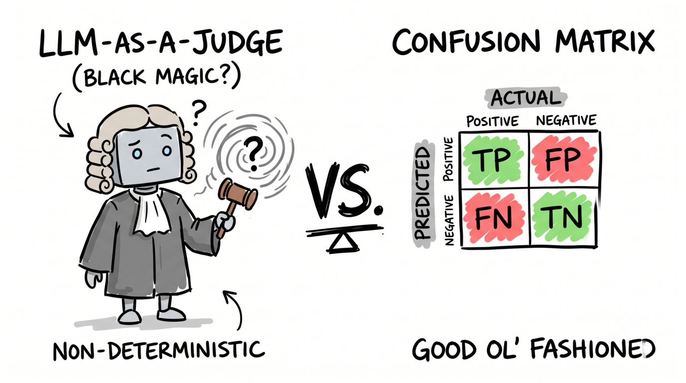
Our team at Miggo Security uses agentic AI for some seriously complicated tasks. When you use a black box like an AI agent to perform a complex task, you start losing sleep over one question - "okay, but is this thing actually working?". Sure, the industry has been sketching out some standards for evaluating agentic features (LLM-as-a-judge and friends), but let's not kid ourselves - none of it hands you the rock-solid confidence you used to get from good old-fashioned Machine Learning. So how do you actually trust what your AI feature is doing? Our approach at Miggo is almost stubbornly old-school: we pretend it's still 2018. Boil every evaluation down to a binary decision question, build yourself a proper baseline dataset, and things suddenly get a lot less mysterious. Getting there isn't always straightforward - but once you crack it, you're standing on much firmer ground.

Recap - What Are Binary Classification Metrics?

If you are familiar with the concept - feel free to skip to the next section

Binary evaluation metrics help us quantify the performance of classification models by comparing predictions against labeled data ("ground truth"). Let's imagine you're building a smart smoke detector that decides whether to sound the alarm based on sensor readings. This is a binary problem - at any given moment, there either is a fire, or there isn't (looking at you, slightly-too-dark toast).

We train our model by running experiments: We create conditions where we know the result, and we compare them to our model’s output. This gives us a matrix of expected vs. actual:

	Actual Positive	Actual Negative
Expected Positive	True Positive	False Positive
Expected Negative	False Negative	True Negative

So every alarm decision falls into one of four buckets:

True positive - there's a fire, and the alarm goes off
False positive - it's just burnt toast, but the alarm goes off anyway
True negative - no fire, and the alarm stays quiet
False negative - there is a fire, but the alarm stays quiet

These are difficult to balance. We would obviously like to have only true positives and true negatives, but we live in a world where that is difficult to achieve. Typically, you need to decide how sensitive your smoke detector is. If you set it to be extra sensitive - it will never miss a real fire, but will also sound the alarm on every burnt toast. Set it to be very insensitive and it will rarely break the silence, but you will probably miss the real fire when it comes.

We want to measure our smoke detector’s quality, to answer the question “is this thing working”. To do that, we need metrics for how to evaluate it. In the binary classification world, these are the most commonly used metrics:

‍Accuracy asks a simple question: out of all of the guesses, how many were correct? This provides a broad (yet shallow) view of model performance. In our example, it measures the detector's overall ability to correctly tell fires and non-fires apart.‍
Precision indicates the quality of positive predictions - specifically, of all the times the alarm went off, how many were real fires? High precision matters because low precision means your household is constantly evacuating the kitchen over a slightly overcooked bagel.‍
Recall measures the model's ability to catch all the actual positive cases - of every real fire that ever happens, how many did the alarm catch? High recall is critical here: missing a real fire (a false negative) is a genuine catastrophe, while a false alarm is just mildly annoying.

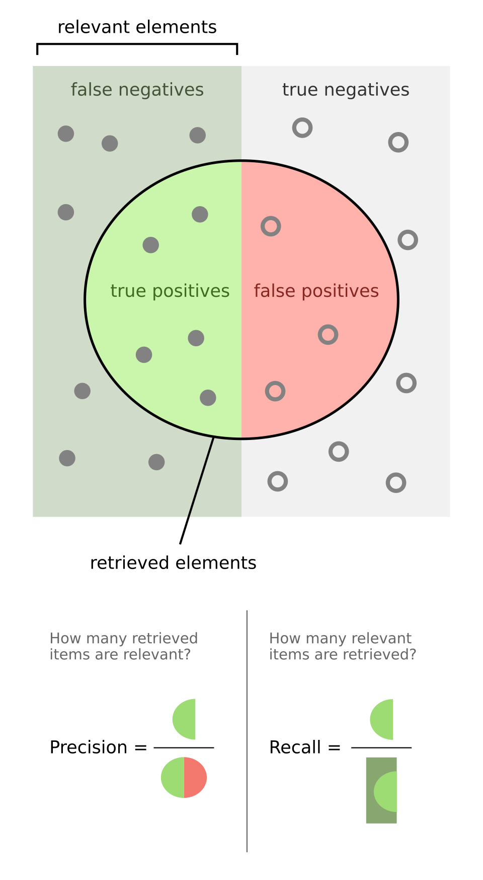
‍Accuracy = (True Positive + True Negative) / (True Positive + True Negative + False Positive + False Negative)‍
Precision = True Positive / (True Positive + False Positive)‍
Recall = True Positive / (True Positive + False Negative)

These seem very similar, yet they’re subtly different - we need all three to get a good understanding of our model’s behaviour. Choosing the most relevant metric to maximize can be very tricky, especially in two very common situations:

When the data is skewed, meaning the ratio of Positive to Negative cases is very far from 1:1. In the smoke detector example, the overwhelming majority of moments in your kitchen involve zero fire. If your detector simply predicts "no fire" for every reading, it could rack up 99.99% accuracy while being completely useless - and dangerous (this great essay on heuristics like this that are right almost all the time and yet provide zero value - he makes the case that a broken smoke detector that never goes off could be "profitably replaced with a rock").
When the costs associated with false positives and false negatives differ. A false positive means an unnecessary evacuation over some toast. A false negative means missing an actual fire, which is a far worse outcome. Therefore, the false negative is the one you really can't afford - recall must be high, even if it costs you some precision.

Different business cases require tuning different metrics - you’re probably not building smoke detectors. Before we draw conclusions from our metrics, it’s important to have a good understanding of what’s important to the business.

So what does all this have to do with LLM-based features? Here are two Miggo features where we applied this technique.

Example 1: WAF Rule Evaluation - Is This Rule Effective for Blocking a Malicious Request?

The Miggo WAF CoPilot feature generates WAF rules that protect your application from security vulnerabilities. If you are new to the field, think of a Web Application Firewall (WAF) as a digital gatekeeper for a website. It sits in front of an application and inspects incoming web traffic to stop malicious activity. WAF rules are the specific instructions or filters that this gatekeeper follows to distinguish between safe, legitimate visitors and harmful requests.

WAF generation seems simple - you give it a vulnerability and you get back a rule as a string. However, building a WAF rule is a task that requires the expertise of an experienced security researcher. How can you trust an AI agent with this? How do you know if it does a fine job? Let’s discuss the evaluation aspect. We have two ways of conducting this evaluation:

LLM-as-a-judge. You feed an LLM the generated rule alongside the context gathered about the vulnerability, and ask it to return a good/bad evaluation. You make sure to prompt with specific questions like “would this rule block a malicious request” and “would this rule block a legitimate request”. This may be trendy, but it gives you non-deterministic results that are difficult to reason about.
You imagine it’s 2018 and do regular old-fashioned data science.

Given how important the WAF CoPilot feature is to us, we chose 2.

‍

Our first step was gathering a baseline dataset. This dataset should be composed of vulnerabilities of interest. It should be diverse enough in every aspect that matters - you may want it to contain various technologies, various attack vectors, or any other characteristic where it is important to properly represent the distribution of vulnerabilities in the real world.

In addition to the vulnerabilities themselves, we gathered relevant payloads. A payload is the content of a request. Certain vulnerabilities can be exploited using very specific malicious payloads, designed specifically to activate the vulnerability. You can find some of these malicious payloads online, available for everyone to use.

Your payloads set should be mixed - some of them malicious (AKA exploits in the cyber jargon), and some of them legitimate. The legitimate payloads are the tricky part - you would want them to be legitimate, but similar enough to the malicious payloads. Trying to “confuse” the LLM is our way of creating and measuring false positives.

The third thing that you need is an instance of a vulnerable demo application protected by WAF. This is your testing mechanism - you can deploy your WAF rule, run an exploit attempt on the vulnerable application, and see for yourself if the attempt succeeded or not. This is a 100% deterministic result and how we classify a rule as succeeding or failing

I know what you may think at this point - setting this up is very time consuming. Well, you are right. But having a reliable evaluation of a key feature is an important enough goal. A big dataset would be great, but even a smaller dataset would give you a more reliable evaluation than the non-deterministic LLM-as-a-judge approach.

Here is how the evaluation process goes:

Run all the payloads (malicious + legitimate) against the vulnerable applications
Keep track of which exploit attempts succeed and which do not. Also - keep track of which legitimate payloads are blocked.
An exploit attempt blocked is a True Positive. A successful exploitation is a False Negative. A legitimate payload blocked is a False positive. A legitimate payload passed is a True negative.
Draw the confusion matrix and analyze the evaluation metrics. Specifically, we are checking Precision as an indicator for the False Positive rate, and Recall as an indicator for the False negative rate.

	Malicious request	Legitimate request
Blocked request	True Positive	False Positive
Successful request	False Negative	True Negative

False Negatives mean that your WAF rules do not protect the application well enough, as too many exploitation attempts manage to get through. In order to minimize their number, you would want to tune the coPilot to create more restrictive rules, which maximizes the recall. False positives mean that your WAF rule is blocking legitimate requests, which means that innocent users do not get served. In order to minimize their number, you would want to tune the coPilot to create more permissive rules, which maximizes the precision. This is a continuous process of tuning the feature, while keeping the tradeoff in mind. As always in the binary classifiers’ world, it is all about the tradeoff.

Example 2: Data Sensitivity Classification - Does this table contain sensitive data?

A second example is data sensitivity classification. We have a feature that uses our visibility to column names for LLM-based labeling of DBs as potentially sensitive, with a closed list of sensitivity categories. Most widely known categories are PII (personal identifiers - e.g addresses, phone numbers), PCI (financial info - e.g cardholder data sensitive authentication data) and PHI (health related info - e.g medical records, treatment data). These are standard categories defined by US regulation. This feature is not a core product value defined by Miggo, but a nice addition on top of the visibility experience that we provide.

In order to evaluate the data sensitivity feature, we focused on specific environments where we had baseline data from a DSPM platform. DSPMs are a product category that has data sensitivity classification as a core feature. We trust that the DSPM products are accurate enough to be used as a baseline. Once you have this data as your ground truth, you can build a confusion matrix that compares your predictions with the DSPM’s data. We created a separate matrix for each sensitivity category.

	DSPM says sensitive	DSPM says not sensitive
Miggo says sensitive	True Positive	False Positive
Miggo says not sensitive	False Negative	True Negative

We mentioned above that balancing precision and recall is tricky. For this feature, we had a clear guideline: No false positives, but false negatives are tolerated. This gives us the privilege to optimize only for precision. It is much easier to tune the feature when your position in the precision-recall tradeoff is so clear, which is very rarely the case.

Summary & Takeaways

The LLM-as-a-judge approach is like black magic - you give it some prompts, it gives you an answer. While often very convenient and appealing to use, it has two major disadvantages:

The results are non-deterministic
For highly complex tasks that require real expertise, it is still not as capable as a human being (as of summer 2026. If you read this in the future - things may change 🙂). Cyber security products still need some human love.

For these reasons, we find that sometimes the human-labeled data approach is still irreplaceable - You get high-quality and deterministic results. You just have to work hard to set everything up this way.

The main challenge that our approach introduces is collecting the baseline datasets. In the WAF CoPilot case, it takes some hands-on time by security researchers, which are a very expensive resource. In the data sensitivity case, we had to actively search a dataset from a DSPM product. This is not just about collecting some dataset. As always in statistical techniques, it should properly represent the population of interest. High quality dataset is always the key.

<script src="https://cdn.jsdelivr.net/npm/gsap@3.12.5/dist/gsap.min.js"></script>
<script src="https://cdn.jsdelivr.net/npm/gsap@3.12.5/dist/Flip.min.js"></script>

<script>
  document.addEventListener("DOMContentLoaded", (event) => {
    gsap.registerPlugin(Flip);
    const state = Flip.getState("");
    const element = document.querySelector("");
    element.classList.toggle("");
    Flip.from(state, {
      duration: 0,
      ease: "none",
      absolute: true,
    });
  });
</script>

<script src="https://cdn.jsdelivr.net/npm/gsap@3.12.5/dist/gsap.min.js"></script>
<script src="https://cdn.jsdelivr.net/npm/gsap@3.12.5/dist/Flip.min.js"></script>

<script>
  document.addEventListener("DOMContentLoaded", (event) => {
    gsap.registerPlugin(Flip);
    const state = Flip.getState("");
    const element = document.querySelector("");
    element.classList.toggle("");
    Flip.from(state, {
      duration: 0,
      ease: "none",
      absolute: true,
    });
  });
</script>